
Laws of Large Numbers and Central Limit Theorem
Published in Fall, 2024
Law of Large Numbers
The law of large numbers has a very central role in probability and statistics. It states that if you repeat an experiment independently a large number of times and average the result, what you obtain should be close to the expected value. There are two main versions of the law of large numbers. They are called the weak and strong laws of the large numbers. The difference between them is mostly theoretical. In this section, we state and prove the weak law of large numbers (WLLN). Before discussing the WLLN, let us define the sample mean.
Another common notation for the sample mean is $M_n$, if the $X_i$’s has CDF $F_X(x)$, we might show the sample mean by $M_n(X)$ to indicate the distribution of the $X_i$’s.
The sample mean, $\overline{X} = M_n(X)$ is also a random variable and we have
\[\mathbb{E}[\overline{X}] = \mathbb{E}[X] \hspace{2cm} \mathbf{Var}(\overline{X}) = \frac{\mathbf{Var}(X)}{n}\]To see this, we have
\[\mathbb{E}(\overline{X}) = \frac{\mathbb{E} X_1 + \mathbb{E} X_2 + \cdots +\mathbb{E} X_n }{n} = \frac{n\mathbb{E} X}{n} = \mathbb{E} X.\]and
\[\begin{align*} \mathbf{Var}(\overline{X}) &= \frac{\mathbf{Var}(X_1+X_2+\cdots+X_n)}{n^2} \hspace{2cm} \text{(since $\mathbf{Var}(aX) = a^2 \mathbf{Var}(X)$)} \\ &= \frac{\mathbf{Var}(X_1) + \cdots +\mathbf{Var}(X_n)}{n^2}\\ & = \frac{n \mathbf{Var}(x)}{n^2} \\ &= \frac{\mathbf{Var}(X)}{n}. \end{align*}\]Click to show/hide proof
If $\mathbf{Var}(X) = \sigma^2 < +\infty$, then we may apply Chebyshev's inequality directly: $$ \mathbb{P}\{ \vert \overline{X} - \mu \vert \geq \epsilon \} \leq \frac{\mathbf{Var}(\overline{X})}{\epsilon^2} = \frac{\mathbf{Var}(X)}{n \epsilon^2} \to 0, \text{as $n \to +\infty$}. $$
Click to show/hide proof
We first observe that $$ S_n^2 = \frac{1}{n} \sum_{i=1}^n (X_i - \overline{X}_n)^2 = \frac{1}{n} \sum_{i=1}^n X_i^2 - \overline{X}_n^2. $$ According to the law of large numbers, we have $$ \frac{1}{n} \sum_{i=1}^n \overline{X}_i^2 \overset{P}{\to} \mathbb{E}(X^2) $$ Also given that $\mathbb{E} X^2 = \sigma^2 + \mu^2$, thus $$ \frac{1}{n} \sum_{i=1}^n X_i^2 \overset{P}{\to} \sigma^2 + \mu^2. $$ Also, by $LLN$, $\overline{X}_n \overset{P}{\to} \mu$, and by continuous mapping theorem, we have $$ \overline{X}_n^2 \overset{P}{\to} \mu^2. $$ So we have $$ \frac{1}{n} \sum_{i=1}^n X_i^2 \overset{P}{\to} \sigma^2+\mu^2 \hspace{0.5cm} \text{and} \hspace{0.5cm} \overline{X}_n^2 \overset{P}{\to} \mu^2 $$ Therefore $$ S_n^2 \overset{P}{\to} (\sigma^2+\mu^2) - \mu^2 = \sigma^2, \text{as $n \to +\infty$}. $$
Central Limit Theorem
Click to show/hide proof
Assume $\{ X_1,X_2,\cdots\}$ are i.i.d random variables with mean $\mu$ and finite variance $\sigma^2$, then the sum $X_1 + \cdots +X_n$ has mean $n \mu$ and variance $n \sigma^2$, consider $$ Z_n = \frac{X_1+X_2+\cdots+X_n - n \mu}{\sqrt{n \sigma^2}} = \sum_{i=1}^n \frac{X_i - \mu}{\sqrt{n \sigma^2}} = \sum_{i=1}^n \frac{1}{\sqrt{n}} Y_i $$ where we define $Y_i = \frac{X_i - \mu}{\sigma}$, each with $0$ mean and unit variance ($\mathbf{Var}(Y) = 1$). The characteristic function of $Z_n$ is given by $$ \phi_{Z_n}(t) = \left[\phi_{Y_1} \left( \frac{t}{\sqrt{n} }\right)\right]^n $$ Given the fact that they are i.i.d. Then the characteristic function of $Y_1$ is, by Taylor's theorem, $$ \phi_{Y_1} \left( \frac{t}{\sqrt{n}} \right) = 1 - \frac{t^2}{2n} + o\left( \frac{t^2}{n} \right), \hspace{0.3cm} \left( \frac{t}{\sqrt{n}} \right) \to 0. $$ where $o(\cdot)$ is the little $o$ notation for some function $t$ that goes to zero more rapidly than $\frac{t^2}{n}$ does. Also since $$ e^x = \lim_{n \to +\infty} \left( 1 + \frac{x}{n} \right)^n $$ we then have $$ \phi_{Z_n}(t) = \left( 1 - \frac{t^2}{2n} + o \left( \frac{t^2}{n} \right) \right)^n \to e^{-\frac{1}{2} t^2}, \hspace{0.3cm} n \to +\infty $$ All of the higher terms vanish in the limit $n \to +\infty$, the right hand side equals the characteristic function of a standard normal distribution ${N}(0,1)$.
An interesting fact about CLT is that it does not matter what the distribution is. To get a feeling of the CLT, let’s first assume that $X_i$’s are $Bernoulli(p)$, then $E X_i = p$, $\mathbf{Var}(X_i) = p(1-p)$, also $Y_n = X_1+\cdots+X_n$ has $Binomial(n,p)$ distributions, thus
\[Z_n = \frac{Y_n - np}{\sqrt{np(1-p)}}\]The figure below shows the PMF of $Z_n$ for different values of $n$, the shape of the PMF gets closer to a normal PDF as $n$ increases.
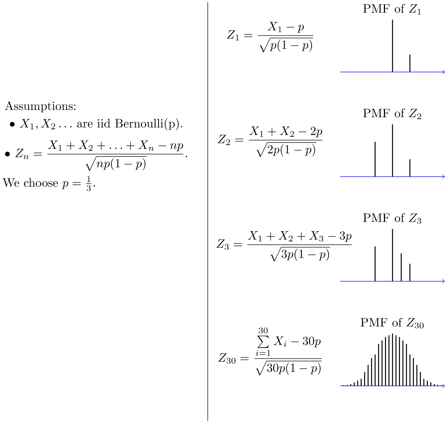
Figure: Illustration of the central limit theorem
As another example, let’s assume that $X_i$’s are $Uniform(0,1)$, then $E X_i = \frac{1}{2}$, $\mathbf{Var}(X_i) = \frac{1}{12}$, in this case
\[Z_n = \frac{X_1+\cdots+X_n - \frac{n}{2}}{\sqrt{n/12}}\]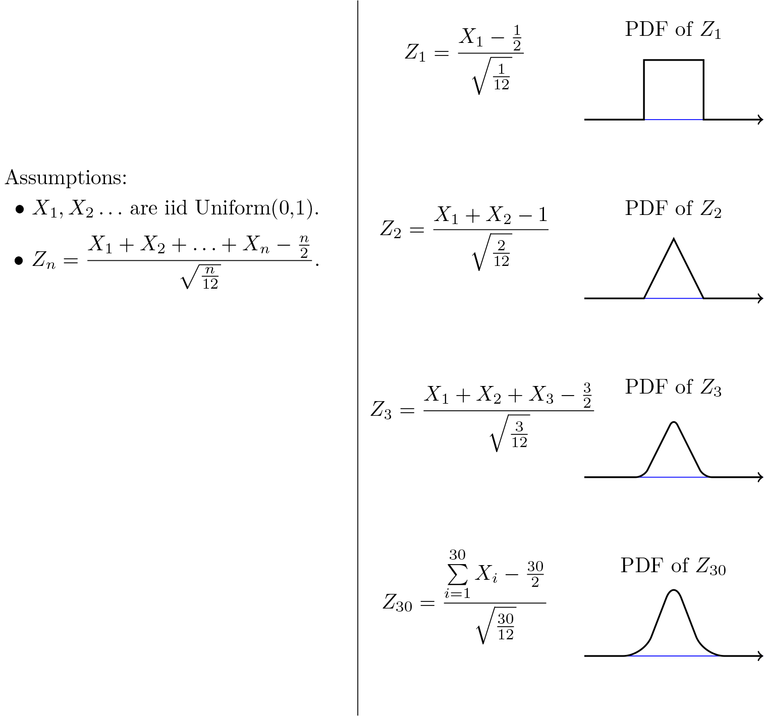
Figure: Illustration of the central limit theorem
The importance of the central limit theorem stems from the fact that, in many real applications, a certain random variable of interest is a sum of a large number of independent random variables. In these situations, we are often able to use the CLT to justify using the normal distribution. Examples of such random variables are found in almost every discipline. Here are a few:
Laboratory measurement errors are usually modeled by normal random variables;
In communication and signal processing, Gaussian noise is the most frequently used model for noise;
In finance, the percentage changes in the prices of some assets are sometimes modeled by normal random variables;
When we do random sampling from a population to obtain statistical knowledge about the population, we often model the resulting quantity as a normal random variable.
Here is the steps that we need in order to apply the CLT:
- Write the random variable of interest, $Y$ as the sum of $n$ i.i.d random variables $X_i$’s:
- Find $\mathbb{E} Y$ and $\mathbf{Var}(Y)$ by noting that
where $\mu = \mathbb{E} X_i$ and $\sigma^2 = \mathbf{Var}(X_i)$.
- According to CLT, conclude that
is approximately standard normal, thus to find $\mathbb{P}{ y_1 \leq Y \leq Y_2 }$, we can write
\[\begin{align*} \mathbb{P}\{ y_1 \leq Y \leq Y_2 \} &= \mathbb{P} \left( \frac{y_1 - n \mu}{\sigma \sqrt{n}} \leq \frac{Y - n \mu}{\sigma \sqrt{n}} \leq \frac{y_2 - n \mu}{\sigma \sqrt{n}} \right) \\ & \approx \Phi \left( \frac{y_2 - n \mu}{\sigma \sqrt{n}} \right) - \Phi \left( \frac{y_1 - n \mu}{\sigma \sqrt{n}} \right). \end{align*}\]where $\Phi$ is the standard normal CDF given by
\[\Phi(x) = \int_{-\infty}^x \frac{1}{\sqrt{2\pi}} e^{-\frac{y^2}{2}} dy\]Click to show/hide solution
Following the steps mentioned above, let $$ Y = X_1 +X_2 + \cdots + X_n $$ where $n=50, \mathbb{E} X_i = \mu = 2, \mathbf{Var}(X_i) = \sigma^2 = 1$, thus we can write $$ \begin{align*} \mathbb{P} \{ 90 < Y < 110 \} &= \mathbb{P} \left\{ \frac{90-n\mu}{\sigma\sqrt{n}} < \frac{Y - n\mu}{\sigma\sqrt{n}} < \frac{110-n \mu}{\sigma \sqrt{n}} \right\} \\ & = \mathbb{P} \left\{ \frac{90-100}{\sqrt{50}} < \frac{Y - n\mu}{\sigma\sqrt{n}} < \frac{110-100}{\sqrt{50}}\right\} \\ & = \mathbb{P} \left\{ -\sqrt{2} < \frac{Y -n \mu}{\sigma \sqrt{n}} < \sqrt{2} \right\} \end{align*} $$ By CLT, $\displaystyle{\frac{Y-n\mu}{\sigma\sqrt{n}}}$ is approximately standard normal, so we can write $$ \mathbb{P}(90 < Y < 110) \approx \Phi(\sqrt{2}) - \Phi(-\sqrt{2}) = 0.8427. $$
Click to show/hide solution
Let's define $X_i$ as the indicator random variable for the $i$th bit in the packet. That is, $X_i =1$ if the $i$th bit is received in error, and $X_i = 0$ otherwise. Then the $X_i$'s are i.i.d. and $X_i \sim Bernoulli(p = 0.1)$. If $Y$ is the total number of bit errors in the pocket, we have $$ Y = X_1 + X_2 + \cdots + X_n $$ Since $X_i \sim Bernoulli(p = 0.1)$, then we have $$ \mathbb{E} X_i = \mu = p = 0.1 ; \mathbf{Var}(X_i) = \sigma^2 = p(1-p) = 0.09 $$ By CLT, we have $$ \begin{align*} \mathbb{P}\{ Y > 120\} & = \mathbb{P} \left\{ \frac{Y - n\mu}{\sigma \sqrt{n}} > \frac{120 - n \mu}{\sigma \sqrt{n}}\right\} \\ &= \mathbb{P}\left\{ \frac{Y - n\mu}{\sigma\sqrt{n}} > \frac{120-100}{90} \right\} \\ &\approx 1 - \Phi\left(\frac{20}{\sqrt{90}} \right)\\ &= 0.0175. \end{align*} $$ In general, if $\sigma$ is not easy to calculate, we can approximate $\sigma$ by $S_n$, which we introduced earlier. We have $$ S_n \overset{P}{\to} \mu. $$ So we have $$ \frac{\overline{X}_n - \mu}{S_n / \sqrt{n}} = \left( \frac{\sigma}{S_n} \right) \left( \frac{\overline{X_n} - \mu }{\sigma / \sqrt{n}} \right). $$
Recommended citation: Jiajun Zhang, (2024) Laws of Large Numbers and Central Limit Theorem