
Multiple and Independent Random Variables
Published in Fall, 2024
Multiple Random Variables
And we claim the following properties:
$F_{\mathbf{X}}$ is non-decreasing in every argument $x_1,x_2,\cdots,x_n$;
$F_{\mathbf{X}}$ is right continuous in all arguments $x_1,x_2,\cdots,x_n$;
$F_{\mathbf{X}} (-\infty,x_2,\cdots,x_n) = F_{\mathbf{X}} (x_1,-\infty,x_3,\cdots,x_n) = \cdots = 0$;
$F_{\mathbf{X}} (+\infty,+\infty,\cdots,+\infty) = 1$;
Let $n=2$, $\forall \epsilon_1,\epsilon_2 >0$, we have
This idea can also be generalized for $n\geq 2$.
For better notation and simplification, we will discuss the case when $n=2$ from now on.
We also give the definition for the continuous type:
We know that $f(x,y) \geq 0$, also
\[\int_{-\infty}^{+\infty} \int_{-\infty}^{+\infty} f(x,y) dudv = 1\]And in particular if $f$ is twice continuous at $(x,y)$, then we have
\[\frac{\partial^2 F(x,y)}{\partial x \partial y} = f(x,y)\]Suppose a $2$-dimensional random variable $(X,Y)$, assume it is of the continuous type, then we define
\[F_1(x) = \mathbb{P}(X_1 \leq x) = F(x,+\infty) = \lim_{y \to \infty} F(x,y)\]and
\[\lim_{y \to \infty} F(x,y) = \lim_{y \to \infty} \mathbb{P} \{ X \leq x, Y \leq y \}.\]Likewise,
\[F_2(y) = F(+\infty,y) = \lim_{x \to \infty} F(x,y)\]and
\[\lim_{x \to \infty} F(x,y) = \lim_{x \to \infty} \mathbb{P}\{ X \leq x , Y \leq y \}\]Also we have
\[f_1(x) = \int_{-\infty}^{+\infty} f(x,y) dy ; f_2(y) = \int_{-\infty}^{+\infty} f(x,y) dx\]We have $f_1(x), f_2(y) \geq 0$, and $f_1(x)$ is called the marginal probability density function of $X$, and $f_2(y)$ is called the marginal probability density function of $Y$.
Now for discrete type, assume $X = { x_1,x_2,\cdots }, Y = { y_1,y_2,\cdots }$, then
\[F(x ,+\infty) = \sum \sum_{(i,j)\in B} p_{ij}, \hspace{0.2cm} B = \{ (i,j) : X_i \leq x , y_j \leq +\infty \}\] \[f_1(x_i) = \mathbb{P}(X = x_i) = \sum_{j=1}^{+\infty} \mathbb{P}(X = x_i), Y = y_j) = \sum_{j=1}^{+\infty} p_{ij} = p_{i \cdot}\]Likewise,
\[f_2(y_j) = \mathbb{P}(Y = y_j) = \sum_{i=1}^{+\infty} p_{ij} = p_{\cdot j}\]Likewise, $p_{i \cdot}$ is called the marginal probability mass function of $X$, and $p_{\cdot j}$ is called the marginal probability mass function of $Y$.
Click to show/hide solution
The marginal distribution of $X$ is given by $$ \begin{align*} f_X(x) &= \int_{-\infty}^{+\infty} \frac{1}{\pi R^2} dy \\ & = \frac{1}{\pi R^2} \int_{-\sqrt{R^2-x^2}}^{\sqrt{R^2-x^2}} dy \\ & = \frac{2}{\pi R^2} \sqrt{R^2 - x^2}, \text{where $x^2 \leq R^2$}. \end{align*} $$ and is equal to $0$ otherwise. Likewise, we have $$ f_Y(y) = \frac{2}{\pi R^2} \sqrt{R^2 - y^2}, \text{where $y^2 \leq R^2$}. $$ and is equal to $0$ otherwise. Since the distace is always non-negative, thus we have $$ \begin{align*} \mathbb{P}\{ \sqrt{X^2 + Y^2} \leq a \} &= \mathbb{P}\{ X^2 + Y^2 \leq a^2 \} \\ &= \iint_{x^2 + y^2 \leq a^2} f(x,y) dxdy\\ & = \frac{1}{\pi R^2} \iint_{x^2+y^2 \leq a^2} dxdy\\ & = \frac{\pi a^2}{\pi R^2} \\ & = \left( \frac{a}{R} \right)^2. \end{align*} $$ So we know that $F_D(a) := \frac{a^2}{R^2}$, so $$ f_D(a) = \frac{2a}{R^2}, 0 \leq a \leq R $$ Hence $$ \mathbb{E} D = \frac{2}{R^2} \int_0^R a^2 da = \frac{2R}{3} $$
Suppose $(X,Y)$ be jointly distributed with joint probability density function given by $f(x,y) = 2, 0<x<y<1$, and $f(x,y) = 0$ otherwise. Then we have
\[f_1(x) = \int_x^1 2 dy = \begin{cases} 2-2x, 0<x<1 \\ 0,\text{otherwise} \end{cases}\] \[f_2(y) = \int_0^y 2 dx = \begin{cases} 2y, 0<y<1 \\ 0, \text{otherwise} \end{cases}\]By definition, we also have
\[p_{i \vert j} = \frac{p_{ij}}{p_{\cdot j}}\] \[F_{X \vert Y} (x,y) = \mathbb{P}(X \leq x \vert Y = y) = \frac{\mathbb{P}(X \leq x, Y = y)}{\mathbb{P}(Y=y)}\]For a continuous random variable, we have
\[\begin{align*} F_{X \vert Y} (x \vert y) &= \mathbb{P} (X \leq x \vert Y = y) \\ & = \lim_{\epsilon \to 0+} \mathbb{P} (X \leq x \vert Y \in (y - \epsilon, y + \epsilon)) \\ & = \lim_{\epsilon \to 0+} \frac{\mathbb{P}(X \leq x , Y \in (y-\epsilon, y+\epsilon))}{\mathbb{P}(Y \in (y - \epsilon, y+\epsilon))}\\ & = \lim_{\epsilon \to 0+} \left( \frac{\displaystyle{\int_{-\infty}^x \int_{y-\epsilon}^{y+\epsilon} f(u,v) dudv}}{\displaystyle{\int_{y-\epsilon}^{y+\epsilon} f_2(v) dv}} \right)\\ & = \frac{\displaystyle{\int_{-\infty}^x f(u,y) du}}{f_2(y)} = \int_{-\infty}^x \frac{f(u,y)}{f_2(y)}du \end{align*}\]and thus
\[f_{X \vert Y} (x,y) = \frac{f(x,y)}{f_2(y)}\]is called the conditional probability density function of the random variable of the continuous type.
Note that
\[\int_{-\infty}^x f(u,y) du = f_2(y) F_{X \vert Y}(x \vert y)\]so we have
\[F_1(x) = \int_{-\infty}^{+\infty} \left[ \int_{-\infty}^x f(u,y) du \right] dy = \int_{-\infty}^{+\infty} f_2(y) F_{X \vert Y}(x \vert y) dy\]where $F_1(x)$ is the marginal distribution function of $X$.
Independent Random Variables
Click to show/hide solution
If we let $X,Y$ denote, respectively the time past $12$ that the man an the woman arrive, then $X,Y$ are independent random variables and each of which is uniformly distributed over $[0,60]$. The desired probability is given by $$ \mathbb{P}\{ X + 10 < Y \} + \mathbb{P}\{ Y + 10 < X\} $$ And by symmetry, is just $2\mathbb{P}\{ X + 10 < Y\}$, thus we have $$ \begin{align*} 2\mathbb{P}\{ X+10<Y\} &= 2 \iint_{x+10<y} f(x,y) dxdy \\ &= 2 \iint_{x+10<y} f_X(x) f_Y(y) dxdy\\ & = 2 \int_{10}^{60} \int_{0}^{y-10} \left( \frac{1}{60} \right)^2 dxdy\\ & = \frac{25}{36}. \end{align*} $$
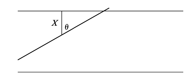
Figure: The Buffon's neddle problem
Click to show/hide solution
Let $X$ be the distance from the middle point of the needle to the nearest parallel line, and $\theta$ be the angle of the needle and the projected line of length $X$. Then by the construction, the needle will intersect the line if and only if $$ \frac{X}{\cos(\theta)} < \frac{L}{2} $$ And we see that $X \in [0,D/2]$ and $\theta \in [0,\pi/2]$, so we may assume that they are independent, and uniformly distributed throughout their ranges, hence we have $$ \begin{align*} \mathbb{P} \left\{ X < \frac{L}{2}\cos(\theta) \right\} &= \iint_{x < \frac{L}{2} \cos(y)} f_X(x) f_{\theta}{y} dxdy \\ & = \frac{4}{\pi D} \int_0^{\pi/2} \int_{0}^{\frac{L}{2} \cos(y)} dxdy\\ & = \frac{2L}{\pi D}. \end{align*} $$
Click to show/hide solution
Since $$ f_{X,Y,Z} (x,y,z) = f_X(x) f_Y(y)f_Z(z) = 1, \hspace{0.1cm} (x,y,z) \in [0,1]^3, $$ so we have $$ \begin{align*} \mathbb{P}\{ X \geq YZ \} &= \iiint_{x \geq yz} f_{X,Y,Z}(x,y,z) dxdydz \\ &= \int_{0}^1 \int_0^1 \int_{yz}^1 dxdydz\\ &=\frac{3}{4}. \end{align*} $$ Suppose $X,Y$ are independent random variables, we also want to find the probability distribution of $X+Y$. We have $$ \begin{align*} F_{X+Y}(a) &= \mathbb{P}\{ X + Y \leq a\}\\ &=\iint_{x+y\leq a} f_X(x) f_Y(y) dxdy\\ &= \int_{-\infty}^{+\infty} \int_{-\infty}^{a-y} f_X(x) f_Y(y) dxdy\\ & = \int_{-\infty}^{+\infty} \int_{-\infty}^{a-y} f_X(x) dx f_Y(y)dy\\ &= \int_{-\infty}^{+\infty} F_X(a-y) f_Y(y)dy \end{align*} $$ The cumulative distribution function $F_{X+Y}$ is called the convolution of the distributions $F_X$ and $F_Y$, by differentiating the equation, we get $$ f_{X+Y}(a) = \int_{-\infty}^{+\infty} f_X(a-y) f_Y(y) dy $$
Click to show/hide solution
We know that $$ f_X(a) = f_Y(a) = \begin{cases} 1, 0<a<1 \\ 0, \text{otherwise} \end{cases}, $$ so we have $$ f_{X+Y}(a) = \int_0^1 f_X(a-y) f_Y(y) dy = \int_0^1 f_X(a-y) dy $$ For $0 \leq a \leq 1$, we have $$ f_{X+Y}(a) = \int_0^a dy = a $$ and for $1 \leq a \leq 2$, we have $$ f_{X+Y}(a) = \int_{a-1}^1 dy = 2-a $$ Hence $$ f_{X+Y}(a) = \begin{cases} a, 0 \leq a \leq 1 \\ 2 - a , 1<a<2 \\ 0, \text{otherwise} \end{cases}. $$
Based on example above, what is the expected number of $n$ such that $X_1+X_2+\cdots+X_n >1$? That is, we want to find
\[N := \min \{ n : X_1 + X_2+ \cdots+X_n > 1 \}\]Note that $N > n$ if and only if $X_1+X_2+\cdots+X_n \leq 1$, so
\[\mathbb{P}\{ N > n\} = F_n(1) = \frac{1}{n!}, \hspace{0.2cm} n>0,\]thus
\[\mathbb{P}\{ N = n\} = \mathbb{P}\{ N > n-1\} - \mathbb{P}\{ N >n\} = \frac{1}{(n-1)!} - \frac{1}{n!} = \frac{n-1}{n!}\]Therefore
\[\mathbb{E}(N) = \sum_{n=1}^{+\infty} \frac{n(n-1)}{n!} = \sum_{n=2}^{+\infty} \frac{1}{(n-2)!} = e.\]The sum of the independent random variables can also be calculated using moment generating functions. Suppose $X_1,X_2,\cdots,X_n$ are $n$ independent random variables and
\[Y = X_1+X_2+\cdots+X_n\]Then
\[\begin{align*} M_Y(s) &= \mathbb{E}[ e^{sY} ] \\ & = \mathbb{E}[ e^{s(X_1+\cdots+X_n)}]\\ &= \mathbb{E}[ e^{sX_1} e^{sX_2} \cdots e^{sX_n}\\ &= \mathbb{E}[e^{sX_1}] \cdots \mathbb{E}[e^{sX_n}]\\ &= M_{X_1}(s) \cdots M_{X_n}(s). \end{align*}\]This important application can be used to find the moment generating function for a binomial random variable. Suppose $X \sim Binomial(n,p)$, then we know that
\[X = X_1+X_2+\cdots+X_n\]where $X_i \sim Bernoulli(p)$, thus
\[M_X(s) = M_{X_1}(s) \cdots M_{X_n}(s)\]where
\[M_{X_i}(s) = \mathbb{E}[e^{sX_i}] = pe^s + 1-p\]So
\[M_X(s) = (pe^s+1-p)^n.\]Recommended citation: Jiajun Zhang, (2024) Multiple and Independent Random Variables